![]()
(4.1)
![]() ,
,
(4.2)
“All motion is an illusion.”
— Zeno of Elea (5th century BCE) —
How separate stars in a galaxy interact? In this chapter, I will show how to simulate the effect of a gravitational field and of Newton’s laws of motion to move stars (simplified to mass bodies) around. The method is referred to as many-body problem, particle simulation, N-body simulation, N-particle simulation or N-body problem[33].
Dynamics is interested in more than a pure description of motion. Dynamics is a study of how a system of bodies evolves over time under the presence of force. Bodies are represented by mass particles (or mass points) that are under the influence of force. The N-body simulation is used to determine the evolution of N-body system.
The N-body simulations can be used in theoretical studies of the large-scale structure of the universe, galaxies, star clusters, solar systems, stellar dynamics, climate modeling, gases, liquids and plasmas. On smaller scales, quantum effects become important. N-body simulations are applied in a wide range of areas outside physics such as N-body simulations of large biomolecules, for example realistic protein unfolding or even simulations of deoxyribonucleic acid (DNA). The N-body simulation has proven to be one of the most versatile methods.
The N-body problem is defined as follows. We have initial conditions i.e. initial positions and initial velocities of all bodies in the system. Interactions (forces) between all bodies in the system have to be evaluated to receive new positions and new velocities. This evaluation is performed repeatedly so that we are getting information about the time evolution of the system.
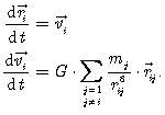
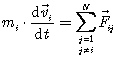
Mathematically is the N-body problem formulated by the system of ordinary differential equations (ODE) coming from Newton’s laws of motion expressed as
|
|
(4.1) |
|
|
(4.2) |
where ![]() ,
, ![]() and
and ![]() are the mass, position and
velocity of the i-th particle, respectively, and
are the mass, position and
velocity of the i-th particle, respectively, and ![]() . The force
. The force ![]() is usually the sum of
external forces. When dealing with molecules, Lennard-Jones force, van der
Waals force or Coulomb’s electrostatic force is used. When dealing with systems
of stars or stellar systems, we will use Newton’s gravitational force[34].
is usually the sum of
external forces. When dealing with molecules, Lennard-Jones force, van der
Waals force or Coulomb’s electrostatic force is used. When dealing with systems
of stars or stellar systems, we will use Newton’s gravitational force[34].
4.2 Gravitational N-body problem
Galaxies are controlled by the force of gravity that acts between all bodies except of self-interaction. First, we will look onto a straightforward application of Newton’s law of gravity and then on a complex hierarchical approximation.
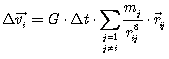
Gravity interaction between all pairs of bodies (except of self-interaction) will introduce a sum to the right side of Equation (4.2) and will become
|
|
(4.3) |
A force ![]() given
by Newton’s universal law of gravitaty, is given by
given
by Newton’s universal law of gravitaty, is given by
|
|
(4.4) |
where ![]() is Newton’s gravitational constant,
is Newton’s gravitational constant, ![]() ,
, ![]() and
and ![]() .
.
After plugging a term for the velocity ![]() (Eq. 4.1) to the left side
of Eq. (4.2), Equation 4.4 is
simplified to a form, where the acceleration
(Eq. 4.1) to the left side
of Eq. (4.2), Equation 4.4 is
simplified to a form, where the acceleration ![]() is
independent on the mass of selected body i
is
independent on the mass of selected body i
|
|
(4.5) |
A dynamical evolution of the system composed of N bodies under the influence of gravity is not solvable to exact solution for more than two bodies[35]. Therefore, a numerical approach is required to study this problem.
4.3 Numerical techniques for solving ODEs
The new position and new velocity of i-th
body must be calculated from the known acceleration. Equation (4.5) contains second derivatives and it is
therefore second-order differential equation. However, all higher-order
differential equations can be transformed into a set of first-order
differential equations (e.g. Press et al., 2002). In our case, Equation (4.5) can be rewritten as two first-order
differential equations by introducing a new variable ![]() as follows
as follows
|
|
(4.6) |
As can be seen, the variable ![]() is the velocity. We already
had both equations (4.6) in (4.1) and (4.3). However, many problems in
computational physics are described by a second order differential equation and
it is useful to know, how they can be semi-automatically reduced to the set of
first-order differential equations. This transformation corresponds in
theoretical mechanics to the Hamiltonian form of equations of motion.
is the velocity. We already
had both equations (4.6) in (4.1) and (4.3). However, many problems in
computational physics are described by a second order differential equation and
it is useful to know, how they can be semi-automatically reduced to the set of
first-order differential equations. This transformation corresponds in
theoretical mechanics to the Hamiltonian form of equations of motion.
We describe laws of physics with continuous
variables and differential equations like Eq. (4.6). However, we must somehow convert
these mathematical equations into a numerical form suitable for a limited
arithmetic of a digital computer. We have to solve differential equations by the
numerical approximation. Let us have some continuous function ![]() in one-dimension and its
numerical representation as shown on Figure 4–1.
in one-dimension and its
numerical representation as shown on Figure 4–1.
![]()

Figure 4–1: A function ![]() tabulated
at discrete time instants
tabulated
at discrete time instants ![]() as values
as values
![]() with timestep
with timestep ![]() .
.
Starting from an initial discrete value ![]() , we can calculate a following
function value
, we can calculate a following
function value ![]() using the equation
for the derivative of a function. The derivative
using the equation
for the derivative of a function. The derivative ![]() of
the function
of
the function ![]() at a given
point
at a given
point ![]() is equal to the slope of
the function
is equal to the slope of
the function ![]() that is
tangent to the function at that given point. It is formally defined as
that is
tangent to the function at that given point. It is formally defined as
|
|
(4.7) |
Here we will approximate the limit by taking
some small, but finite ![]() rather than
mathematically letting it go to zero. Through this very small interval
(timestep)
rather than
mathematically letting it go to zero. Through this very small interval
(timestep) ![]() , a good approximation to the
underlying differential equation is achieved. The derivative at the starting
point of each interval is linearly extrapolated to find the next function
value. We assume that the derivative remains constant in the interval between
, a good approximation to the
underlying differential equation is achieved. The derivative at the starting
point of each interval is linearly extrapolated to find the next function
value. We assume that the derivative remains constant in the interval between ![]() and
and ![]() . Therefore, in order to
solve ODE and find the value
. Therefore, in order to
solve ODE and find the value ![]() at the point
at the point
![]() , we need to know the initial
value
, we need to know the initial
value ![]() at the point
at the point ![]() . This problem involving ODE
is therefore specified not only by its equations, but also by the initial value
and therefore is called the initial value problem[36].
Consequently, an approximate solution to the differential equation is given by the
initial value and the scheme
. This problem involving ODE
is therefore specified not only by its equations, but also by the initial value
and therefore is called the initial value problem[36].
Consequently, an approximate solution to the differential equation is given by the
initial value and the scheme
|
|
(4.8) |
where ![]() . Second
term on the right side of Equation (4.8)
. Second
term on the right side of Equation (4.8) ![]() is
the first term of series in the Taylor expansion of
is
the first term of series in the Taylor expansion of ![]() about
about
![]() . This scheme for numerically
approximating the solution of ODE invented Leonhard Euler[37].
. This scheme for numerically
approximating the solution of ODE invented Leonhard Euler[37].
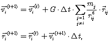
We must now apply Euler’s scheme to equations (4.6) and finally compute the new position
and new velocity of the i-th body. When we consider the change of ![]() to
to ![]() we can express the increments
of the position and velocity as
we can express the increments
of the position and velocity as
|
|
(4.9) |
|
|
(4.10) |
With certain initial conditions this will ultimately change to
|
|
(4.11) |
where ![]() ,
, ![]() are new values of velocity
and position of i-th body and
are new values of velocity
and position of i-th body and ![]() ,
, ![]() are previous values of
velocity and position of i-th body, respectively.
are previous values of
velocity and position of i-th body, respectively.
Although Euler’s method is cheap to compute, it is not very desirable for practical purposes, due to its inaccuracy when compared to other methods. These methods use more points and higher derivatives to get a better estimate of the derivation in the point of interest, which is paid off by the requirement of more computational power.
Nevertheless, we can improve Euler’s method, so
that it is much more accurate and that its computational cost is only slightly
higher. This method uses derivatives computed at the midpoint of each step. In
addition, it avoids the need for computing second derivative. Moreover, the midpoint
method is very well suited for second-order differential systems of type ![]() by design and is therefore
suitable for N-body problem solutions.
by design and is therefore
suitable for N-body problem solutions.
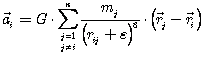
The extra actions taken to prepare the system
for midpoint method are the prediction of the position of body ![]() at the middle of the
timestep
at the middle of the
timestep ![]() according to
according to
|
|
(4.12) |
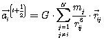
and the acceleration based on this positions at ![]() computed as
computed as
|
|
(4.13) |
Then the i-th particle is advanced according to
|
|
(4.14) |
|
|
(4.15) |
Velocities are one-half of the timestep out of synchrony with positions.
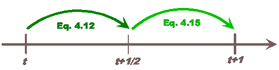
Figure 4–2: The evaluation of position in the midpoint method is looking like a jumping frog. Therefore, this method is also called the leapfrog.
4.4 Methods for solving galactic N-body problem
To solve the N–body problem for large N,
we must look at the efficiency of a computer solution to be sure that
simulation time will not be prohibitive. An algorithm’s efficiency can be
evaluated through the number of computations that must be carried out in order
to solve a given problem. Usually, it is impossible to exactly predict the number
of operations performed by a computer, because it depends on exactly what a machine
or language implementation is being used. Therefore we generally use the “big O”
notation to generalize a computational complexity (“the speed of a program”). The
computational complexity usually depends on the size n of the input data
![]() .
.
Ideally, a dynamical evolution of a galaxy would
be modeled with a direct N-body simulation. In the framework of the
direct N-body simulation, each body interacts with ![]() other bodies. The
interactions must be carried out for each of the N bodies. To compute the
accelerations (4.13) for each
of the N bodies, the direct algorithm must summate over
other bodies. The
interactions must be carried out for each of the N bodies. To compute the
accelerations (4.13) for each
of the N bodies, the direct algorithm must summate over ![]() bodies. In order to evaluate
force interactions of the system composed of the N bodies,
bodies. In order to evaluate
force interactions of the system composed of the N bodies, ![]() computations are needed;
that is nearly
computations are needed;
that is nearly ![]() computations. For a
galaxy with
computations. For a
galaxy with ![]() stars,
stars, ![]() computations are needed. To
study evolutionary stages of such galaxy, we will need at least tens of
thousands of such timesteps. Of course, it is possible to use third Newton’s law of motion, which holds that “to every action there is always opposed an equal
reaction” (Newton, 1687). This reduces the number of required computations to a
half, i.e.
computations are needed. To
study evolutionary stages of such galaxy, we will need at least tens of
thousands of such timesteps. Of course, it is possible to use third Newton’s law of motion, which holds that “to every action there is always opposed an equal
reaction” (Newton, 1687). This reduces the number of required computations to a
half, i.e. ![]() . However, computational
complexity is still
. However, computational
complexity is still ![]() . It means that the
number of computations is approaching
. It means that the
number of computations is approaching ![]() ,
where c is some constant. This direct (brute-force) computation provides
a high accuracy for the price of huge time complexity. Therefore, number of bodies
that can be simulated is dramatically limited.
,
where c is some constant. This direct (brute-force) computation provides
a high accuracy for the price of huge time complexity. Therefore, number of bodies
that can be simulated is dramatically limited.
General-purpose computers are becoming more advanced so that N-body simulations can account with more and more bodies. Computations on a graphics card in personal computer with a high processing speed called GPGPU (General-Purpose computation on Graphics Processing Units) are becoming available. Single-purpose computers like GRAPE (built around specialized pipeline processors, literally “GRAvity PipE”) introduced in 1990 and computers with FPGA (Field Programmable Gate Array) are increasing a widespread usage and the accuracy of N-body simulations.
Advancement not only in the power of computer hardware, but also in the development of sophisticated algorithms made possible studies of large systems of bodies like galaxies or galaxy groups. Still, the gravitational influence is long reaching. Therefore, it is impossible to neglect in computations bodies behind some spatial distance. However, astronomical systems have properties that can be utilized in designing “faster” computational methods. These methods lead to the reduction of required differential equations that must be solved in order to obtain new positions and velocities of bodies in the modeled system. A small error is introduced in exchange for a large speedup.
A lot of methods for a faster simulation of gravitational force was invented. However, it is possible to divide them into two basic groups.
· Methods based on finite differences, finite elements, grid or mesh methods, Eulerian codes – e.g. particle in cell (PIC), particle-mesh (PM), particle-particle/particle mesh (P3M) – computes even in regions with a low number of bodies, grid density same everywhere even in areas without bodies, geometrical restriction, useful mainly for homogenous particle distributions. Used from 1960s: forces are evaluated in each of the cell of the grid; fast Fourier Transform (FFT) is then used to solve the gravitational potential from a density distribution interpolated onto a regular mesh.
· Methods based on a particle system, grid-less methods, Lagrangian codes – adaptive for non-homogenous particle distributions without the loss of speed, does not waste time in regions with a low number of bodies. Invented in 1980s. Tree methods: Once a tree is built, it can be re-used as an efficient search method for other physics such as smoothed particle hydrodynamics (SPH).
State-of-the-art simulation codes like GADGET-2 (Springel, 2005) combine both techniques into a single hybrid code.
4.5 Hierarchical approach to N-body problem
How can we find out the gravitational influence
of the galaxy M31 in the constellation of Andromeda[38] to
the Earth? The number of stars in the Andromeda galaxy is of order ![]() . If we look at this galaxy
on the night sky, we cannot distinguish its individual stars, because of the great
distance of 730 kpc; we see it as a patch of light. The same physical intuition
can be applied to the gravity. If we are computing the gravitational influence
of the distant Andromeda galaxy, we can substitute the whole Andromeda with a single
mass point, which position will be located at the center of mass of that galaxy
(see Figure 4–3).
. If we look at this galaxy
on the night sky, we cannot distinguish its individual stars, because of the great
distance of 730 kpc; we see it as a patch of light. The same physical intuition
can be applied to the gravity. If we are computing the gravitational influence
of the distant Andromeda galaxy, we can substitute the whole Andromeda with a single
mass point, which position will be located at the center of mass of that galaxy
(see Figure 4–3).
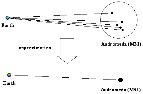
Figure 4–3: Gravitational potential of the distant system of bodies approximated as the potential of a single body.
Barnes and Hut (1986) introduced such a method for solving N-body problem that requires less computation than the direct N-body method. The gravitational influence of distant bodies can be combined into a single group so that the whole group acts as a single body. This method is called the Barnes-Hut algorithm, tree-code, or hierarchical tree-code.
4.6 Building tree hierarchy, space decomposition
A basic computer structure representing a physical spatial distribution of bodies in a space is a tree. The root of the tree (overall simulated volume) encompasses all bodies in the simulated system. The tree is constructed from the root by splitting the simulated volume into rectangular cubes (cells, domains). In three dimensions, the division of the parent cube into eight daughterly cubes (potential new nodes) constructs every node of the tree. The tree structure is therefore called octal-tree or simply oct-tree. The division is accomplished by splitting each of the Cartesian dimension to a half. This repeatedly continues until the cube contains more than one body. If there is only one body in the cube left, it is stored as a leaf in the tree structure. When the cube is empty, it is ignored. The tree is composed of a hierarchical arrangement of leaves, nodes and the root (top-most node) (Figure 4–4). The leave represents the mass point itself, in the hierarchy is on the lowest position. The tree is usually reconstructed during every timestep.
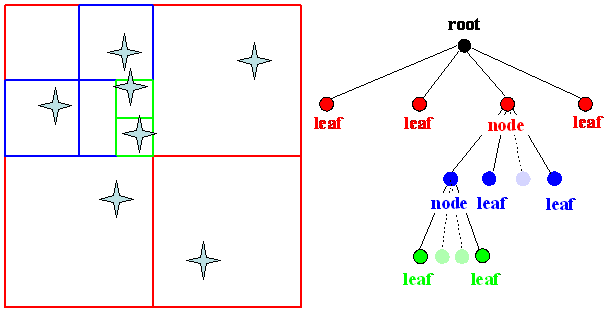
Figure 4–4: A two-dimensional simulation volume with stars is divided to four areas (left). A related quad-tree (right) is constructed in a clockwise pass starting at the bottom-right red square of the simulation volume. Empty squares of the simulated volume are ignored in the tree and are illustrated as transparent circles connected with dotted branches to the parent node.
The tree method is suitable for astronomical systems. It is adaptive to a non-homogenous distribution of bodies, because it automatically adjusts to the particle distribution. In the case of uniform distribution, the tree has the same depth everywhere. On contrary, in a typical galaxy with more stars in the center, the tree is automatically deeper at the center and shallower on the edge (see Figure 4–5). This is the source of troubles for simulations with grid-based codes.
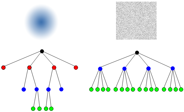
Figure 4–5: Galaxy-like (left) and uniform (right) distributions. The adaptability of the tree method is very useful in galaxy calculations with a highly varying particle distribution.
4.7 Division of space with Hilbert’s space-filling curve
The simulated volume can be optionally divided by a space-filling curve[39]. The space-filling curve completely fills up the simulated volume by passing through the every point of simulated volume. It is physically meaningful to divide the simulated volume continuously.
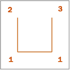
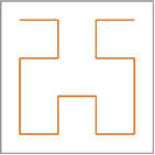
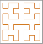
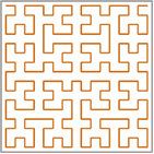
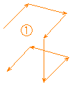
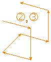
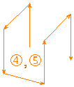
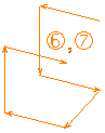
Hilbert’s curve in 2D can be constructed
recursively starting with an initial curve ![]() .
We can identify orientations of the curve
.
We can identify orientations of the curve ![]() with
numbers (1), (2), and (3) (see Figure 4–6). The subsequent curve scheme is determined by the previous through
replacing both (1) with the smaller version of the same orientation of the scheme
and by replacing ends (2, 3) with rotated and mirrored versions of the scheme.
On the next level is applied the same algorithm on each part of the previous scheme.
with
numbers (1), (2), and (3) (see Figure 4–6). The subsequent curve scheme is determined by the previous through
replacing both (1) with the smaller version of the same orientation of the scheme
and by replacing ends (2, 3) with rotated and mirrored versions of the scheme.
On the next level is applied the same algorithm on each part of the previous scheme.
|
|
|
|
|
|
|
|
|
|
Figure 4–6: Pattern of Hilbert’s curve in two dimensions.
In three dimensions, Hilbert’s curve copying is somewhat more complicated. Again, the subsequent orientation of Hilbert’s curve can be determined from its predecessor through a rotation. Let us define the initial orientation of Hilbert’s curve (level 0) as on Figure 4–7. In the following step (level 1), the cube will be divided and traversed with Hilbert’s curve in a way marked in Figure 4–8.

Figure 4–7: The initial orientation of Hilbert’s curve (level 0, root cube) in the three-dimensional simulated volume. The division of this cube will construct level 1 of the oct-tree in a marked way.
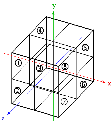
Figure 4–8: Level 1 division of the three-dimensional Hilbert’s curve.
Rules for copying to the subsequent step are now following. Initial Hilbert’s curve (level 0) will be rotated as follows:
1. Rotate around y-axis by ![]() and around x-axis by
and around x-axis by ![]() .
.
2. Rotate around y-axis by ![]() and around z-axis by
and around z-axis by ![]() .
.
3. Same as (2).
4. Rotate around x-axis by ![]() .
.
5. Same as (4).
6. Rotate around y-axis by ![]() and around z-axis by
and around z-axis by ![]() .
.
7. Same as (6).
8. Rotate around y-axis by ![]() and around x-axis by
and around x-axis by ![]() .
.
|
|
|
|
|
|
|
y |
y |
x |
y |
y |
Figure 4–9: The traversal of the simulated volume by Hilbert’s curve.
Every node contains information describing a mass distribution of bodies that fall within this node. Once the tree construction phase is finished, information about a position, velocity and total mass of node’s descendants is computed and stored into each node. This calculation is performed in one pass from leaves to the root. For higher accuracy, quadruple or higher order moments should be also computed. However, such calculations lead to higher requirements on a simulation time and computational slowdown.
The pass through the tree from its root computes force acting on every single body in the system. It will take the body from the current node (for the first time, it is the root node) and it will receive its descendant (nodes or leaves from one of eight possible sub-nodes of the root). If the center of mass of the current node is sufficiently distant from the selected body, the force is computed as the force acting between the selected individual body and the node. This is the heart of the speed-up of force computations.
If the distance between the selected body and the node (its center of mass) is not sufficient then the node is “opened” and a distance check is performed between all of its leaves or sub-nodes and the selected body (see Figure 4–10). This is executed repeatedly. The worst-case scenario is that the algorithm will dig-down all the way from the root to individual leaves (individual bodies) and the computational complexity will be the same as in the case of the direct N-body simulation.
When is the node “sufficiently distant”? A criterion determining sufficient distance is a multipole acceptability criterion or MAC. Barnes and Hut (1986) introduced criterion
|
|
(4.16) |
where d is the distance between the selected
body and the mass center of node, l is the length of cube’s edge (see Figure 4–11) and ![]() is
the opening angle. Parameter
is
the opening angle. Parameter ![]() determines
the speed-up of the algorithm and accuracy at the same time. It is suggested to
choose this parameter in the range
determines
the speed-up of the algorithm and accuracy at the same time. It is suggested to
choose this parameter in the range ![]() (Hernquist,
1987). Smaller values of
(Hernquist,
1987). Smaller values of ![]() are leading
to the opening of a larger number of nodes, to a better accuracy of force
computation and to computational slow-down.
are leading
to the opening of a larger number of nodes, to a better accuracy of force
computation and to computational slow-down.
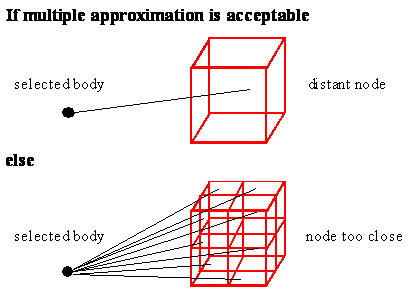
Figure 4–10: If the distance between the selected body and the node is sufficient, the computation of force is performed between them. Otherwise, the distance criterion is applied to all descendants of the node.
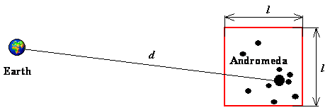
Figure 4–11: The meaning of parameters d and l in the Barnes-Hut criterion.
This approach leads to the reduction of required
interactions and to the decrease of computational complexity to ![]() . It is a substantial
improvement over the direct summation method with
. It is a substantial
improvement over the direct summation method with ![]() complexity (see Figure 4–12). To further improve a performance
and reduce a total processor time required for a simulation run, I parallelized
this part with OpenMP[40].
complexity (see Figure 4–12). To further improve a performance
and reduce a total processor time required for a simulation run, I parallelized
this part with OpenMP[40].
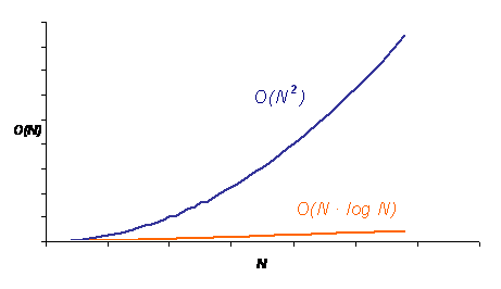
Figure 4–12: A superior scaling ![]() of the hierarchical
method for solving the
of the hierarchical
method for solving the
N-body
problem as compared to the direct method with quadratic ![]() complexity.
For the same number N of
bodies, fewer computations are required with the hierarchical method.
complexity.
For the same number N of
bodies, fewer computations are required with the hierarchical method.
4.10 Grouping
Interaction evaluation and MAC testing are located in the computationally most-intensive part of the algorithm. Therefore, it is convenient to look for optimizations of this time-critical part of code. We can suppose that bodies that are spatially close to each other will interact with the nearly same nodes (Barnes, 1990). We should therefore create groups of close bodies according to their spatial location. We can utilize cubes (nodes) produced during the tree construction. When such encompassing cube contains some limited number of bodies (my simulations used always 32 bodies), we can call it the group and add this group (cube) into the list of groups. During the force evaluation, we do not choose the single body; instead we choose the whole group.
Nodes or leaves interacting with the selected group might be split into two lists (Becciani et al., 2000). The first list contains bodies (nodes or leaves) that are sufficiently distant and affect the group’s center of mass, and therefore all bodies in the selected group. The second list contains bodies that are too close and interaction with them must be computed individually for each body in the group.
Again, we must introduce some criterion that will decide to which list should be the node or leave inserted. We can encompass all bodies in the group with a sphere of radius (Becciani et al., 2000)
|
|
(4.17) |
where c is a parameter determining an accuracy
and ![]() is the length of the cube’s
edge. If the separation
is the length of the cube’s
edge. If the separation ![]() (see Figure 4–13) between the group’s center of
mass and the distant node is greater than
(see Figure 4–13) between the group’s center of
mass and the distant node is greater than ![]() ,
the distant node is inserted to the first list. Otherwise, the distant node is
ascribed to the list of close bodies. Finally, all bodies from the group are
added to the second list.
,
the distant node is inserted to the first list. Otherwise, the distant node is
ascribed to the list of close bodies. Finally, all bodies from the group are
added to the second list.
Parameter c determines the accuracy and
is chosen to be ![]() .
.
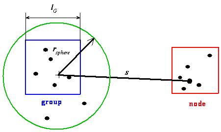
Figure 4–13: The meaning of parameters ![]() ,
, ![]() and
and ![]() in
the grouping strategy.
in
the grouping strategy.
4.11 Exploding galaxies
Galaxies are collisionless systems, which mean that its components (stars) do not affect each other by close encounters. Orbit of a single star is affected almost entirely by an overall potential of the whole galaxy, not by other star that is nearby. On contrary, star clusters are collisional systems, which mean that also the close encounters of bodies (stars) are important in computation and paths of individual bodies might be substantially altered by close passes of neighbors. As the notion suggests, collisional systems are so dense that stars may eventually get so close to each other that they may collide. Therefore, star clusters are sometimes called dense stellar systems. If you are interested in the modeling of dense stellar systems, read Hut and Makino (2006).
While using a constant timestep, two bodies can get very close to each other so that unbearable numerical error is introduced. An integration with an improperly big timestep (therefore called overstep problem) might lead to an anomalously high velocity of a body (star), which as a result leave a gravitationally bound system of bodies. When such encounter occurs in a numerical simulation, the star is unnaturally accelerated and flies out of the galaxy (therefore called disk-heating problem). This is a direct effect of discrete numerical calculations. In differential equation is movement described continuously and smoothly.
Close encounters of stars in a real galaxy are improbable
with regard to a low spatial distribution of stars. In order to treat the
galaxy as the collisionless system, bodies i and j in Equation (4.4) should never get close to each other
(not even during the collision of galaxies). Therefore a gravitational
softening (smoothing) must be employed to avoid nonrealistic acceleration
caused by the close encounters (Aarseth, 1963). Small number called a softening
length ![]() must be added to the denominator
in Newton’s universal law of gravitation (
must be added to the denominator
in Newton’s universal law of gravitation (![]() is
replaced by
is
replaced by ![]() ). The softening length
). The softening length ![]() must be small when compared
to galaxy dimensions. The softening essentially smoothens out microphysics that
cannot be resolved in the simulation. For large distances, the small number
must be small when compared
to galaxy dimensions. The softening essentially smoothens out microphysics that
cannot be resolved in the simulation. For large distances, the small number ![]() has little effect; model is
more collisionless. Stars interact through the customary “softened”
gravitational force where an acceleration
has little effect; model is
more collisionless. Stars interact through the customary “softened”
gravitational force where an acceleration ![]() is
expressed as
is
expressed as
|
|
(4.18) |
A mathematical formulation of the gravitational
force depends on an inverse square of a distance between bodies i and j.
The mass point representing the star is essentially an infinitely deep
potential well that can be expressed as Dirac’s δ‑function[41] in
the point’s location. When these two bodies are very close to each other ![]() , the evaluation of
acceleration together with the large timestep may bring a very large number
that may introduce numerical errors or even lead to infinity. The gravitational
softening will therefore eliminate numerical errors introduced when two bodies
approach each other. Other solution to the close encounter problem is a variable
timestep or cutoff radius, which reduces interaction at short ranges.
, the evaluation of
acceleration together with the large timestep may bring a very large number
that may introduce numerical errors or even lead to infinity. The gravitational
softening will therefore eliminate numerical errors introduced when two bodies
approach each other. Other solution to the close encounter problem is a variable
timestep or cutoff radius, which reduces interaction at short ranges.
4.12 Code limitations
The difference between ![]() and
and ![]() is immense and many more
stars can be simulated. Nevertheless, the real galaxies have billions of stars
and realistic simulations of galaxy dynamics will stay unreachable for some
time. The value of N is too large for a simulation where each body
represents the single star. This number is even beyond the power of modern
computers, the speed of existing computers and sophisticated algorithms is still
too limited for the number of bodies. Therefore, each individual particle in
the simulation represents rather a large association of stars.
is immense and many more
stars can be simulated. Nevertheless, the real galaxies have billions of stars
and realistic simulations of galaxy dynamics will stay unreachable for some
time. The value of N is too large for a simulation where each body
represents the single star. This number is even beyond the power of modern
computers, the speed of existing computers and sophisticated algorithms is still
too limited for the number of bodies. Therefore, each individual particle in
the simulation represents rather a large association of stars.
On contrary, solar system simulations are computed with an interest on specific bodies (planets, moons, asteroids, comets, spaceships) and their particular precise orbit. N-body simulations of galaxies are more of a statistical nature, they do not testify about orbits of individual stars. Individual bodies do not represent individual stars in our galaxy simulation.
The hierarchical and numerical approximation may lead to unacceptable errors in the simulation. Errors increases with each timestep in general. When simulating for several thousand time-steps, these errors will add up. Whatever code we use, we should test it in analytic limits where possible. We should compare our simulations with observations from telescopes and check whether our results are meaningful. We should use our intuition and ask what the output should be. The computer only does what we tell it to do, and will happily perform meaningless simulation. With the impressive power and scope of numerical techniques, we should be always aware of numerous potential pitfalls. Although remarkably robust, numerical simulations must be used with care if the results are to be meaningful. When we start computing, we should be careful and not stop thinking. Yet dynamics in galaxies is worth of study.
4.13 Concluding remarks
In Chapter 4, we have shown how to simulate the effect of the gravitational field and of Newton’s laws of motion to move the stars around. I described my implementation of Barnes-Hut algorithm for many-body simulation and novel geometry-based construction of the 3-dimensional Hilbert’s curve. Simulation code works in four steps. First, a tree is constructed by space decomposition from a list of bodies that form the simulated system. Space is divided utilizing Hilbert’s self-similar space-filling curve. Groups of close bodies are created. Second, centers of mass of individual nodes are computed. Third, accelerations are computed with the Barnes-Hut algorithm. Fourth, new positions and velocities are computed. Thanks to this algorithm, all simulations will be fully self-consistent, i.e. no rigid potentials will be employed.

 .
.